Reservoir

With Piper, you can define numerous types of reservoirs that can be connected to wells. The first four of these reservoirs use material balance techniques. The transient reservoirs use direct solution methods based on the input of reservoir characteristics. The types of reservoirs supported by Piper are the following:

• Volumetric Depletion Reservoir
• Connected Reservoir
• Water Drive Reservoir
• Geo-pressured Reservoir
• Transient Reservoir

Volumetric Depletion (Tank-Type) Reservoir

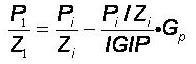
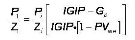
In a Volumetric Depletion Reservoir the internal energy of the gas is the primary drive mechanism that moves the gas towards the surface. As gas is produced from the reservoir, the pressure in the reservoir declines. The relationship between the compressibility adjusted pressure in the reservoir and the cumulative gas produced will follow a straight line. This is often referred to as the P/Z plot. The equation used by Piper to describe the relationship is:

Required Input for Volumetric Depletion Reservoir

The Volumetric Depletion reservoir is the assumed reservoir used by Piper unless the user specifies another reservoir type. Five inputs are required to define a Volumetric Depletion reservoir:

• Original Gas in Place
• Cum Gas to Date
• Original Reservoir Pressure
• Reservoir Temp
• Reservoir Depth
• Recovery Factor

The Original Gas in Place (OGIP) is the gas contained in the reservoir before production began. The Cum Gas to Date is the amount of gas extracted from the reservoir up to the date of the current forecast configuration. The Original Reservoir Pressure is the initial shut-in pressure of the reservoir before production commenced. The current reservoir pressure can be calculated from these three inputs.

The Reservoir Temp is the current temperature of the reservoir. It is used to adjust for temperature dependence of compressibility effects.

The Pool Depth is the depth of the pool, measured to the mid point of perforations.

The Recovery Factor can be used to stipulate the economic recovery limit for the reservoir.

Connected Reservoir

Many gas reservoirs have areas of high permeability that are in communication with surrounding areas of low permeability. This contrast in permeability, which is typical of "tight gas reservoirs", affects the P/Z relationship that the reservoir follows as it depletes.

The existence of such heterogeneity complicates the material balance analysis because the high permeability area will deplete at a faster rate than the low permeability area. The low permeability area will then act as a recharging mechanism to the high permeability area. This interaction renders the material balance plot non-linear (P/Z plot is concave upward).

Often the reserves contained in the low permeability region are significant, and can be larger than those in the high permeability region. The existence of the low permeability region will often affect the depletion profile of the high permeability region. Piper uses the Connected Reservoirs theory to model this behavior.

The connected reservoir can be visualized as two tanks in communication with each other, as shown in the figure below:

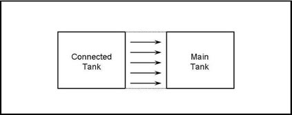
In the connected reservoir model used by Piper production of gas takes place from the main tank only. The connected tank, referred to as the Connecting Reservoir, acts as a low permeability recharging pool. This pool is depleted indirectly into the main tank where production takes place. The pressure behavior of the two communicating tanks is described by a material-balance equation written for each compartment:

 

 

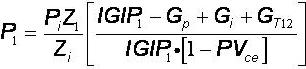
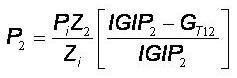
P1 and P2 are the pressures in the main tank and connected tank respectively. The two material-balance equations are coupled through the GT12 term, which represents the cumulative gas influx from the connected tank (designated with the subscript '2') to the main tank (designated with the subscript '1').

The degree of communication between the two tanks is characterized by a transfer relationship. Piper utilizes the following transfer relationship:

where 'C' is the transfer coefficient.

Required Input for Connected Reservoir

To use the Connected Reservoir Module in Piper, three inputs are required.

• Original Gas in Place
• Transfer Coefficient
• Cum Gas Transferred

These inputs all pertain to the connected reservoir. The 'main tank' is defined in the pools menu in the same manner you would define a simple Volumetric Depletion Reservoir.

The Original Gas in Place is the gas contained within the connected reservoir before production commences. The Transfer Coefficient is a constant that defines the transfer of gas from the connected to tank to the main tank. The Cum Gas Transferred is the amount of gas transferred from the connected tank to the main tank up to the date of the current forecast configuration.

The connected reservoir module is most often used for a reservoir that is already exhibiting behavior that deviates from a straight line P/Z plot. In such cases the Transfer Coefficient and Cum Gas Transferred can be adjusted to accurately mimic the P/Z versus Cum relationship being observed. F.A.S.T. MBA™, used along with the production and pressure history for the reservoir, can be used to fit the Connected Reservoir model to the history.

Water Drive Reservoir

Many gas reservoirs are associated with adjacent aquifers from which there is water expansion that encroaches upon the reservoir as gas is produced. Water encroachment provides an important source of pressure support for the reservoir and must be taken into account when performing material balance calculations. The gas expansion dynamics no longer act in isolation to dictate a straight line P/Z versus Cum relationship. Instead, the P/Z plot will trend concave up, with the extent of the concavity being dictated by the strength of pressure support being provided by the underlying aquifer.

The material balance equation for a gas reservoir with water drive accounts for gas expansion characterizing a Volumetric Depletion Reservoir as well as the effect of the influx of water from the adjacent aquifer.

Required Input for Water Drive

The Piper Water Drive requires input of three parameters:

• Aquifer Volume
• Transfer Coefficient
• Cum Water Transferred

Piper treats the influence of the aquifer in a manner similar to the way it treats the influx of gas from a connected reservoir. The influx of water into the reservoir is assumed to follow the following deliverability relationship.

Where 'C' is the Transfer Coefficient.

The aquifer is assumed to initially be at the same pressure as the original reservoir pressure. Because the pressure of the reservoir and that of the aquifer are the same, there is no influx of water into the reservoir for the first time step (either a daily or monthly period) and the reservoir follows a Volumetric Depletion relationship. Beyond the first month, a pressure difference does exist between the reservoir and the aquifer. Thus there will be flow from the aquifer to the reservoir, and that flow will be dictated by the deliverability relationship described above.

At the end of each forecast time step the change in pressure of the aquifer due to the reduction of water within the aquifer is determined by the following compressibility equation:

This equation relates the amount of water transferred during the time step (We), to the initial aquifer volume at the beginning of the time step (Wi), the total rock and water compressibility (c), determined internally by Piper, and the change in pressure of the aquifer during the time step.

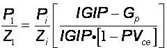
Geo-Pressured Reservoir

In a Geo-Pressured Reservoir, the impact of the compressibility of the connate water and rock cannot be ignored. The expansion of the connate water and rock act as additional drive mechanisms to the primary gas expansion drive mechanism.

The material balance equation for a Geo-Pressured Reservoir accounts not only for the gas expansion characterizing a Volumetric Depletion Reservoir but as well for the expansion of the rock and water:

Required Input for Geo-Pressured Reservoir

The Piper Geo-Pressured Reservoir module requires input of two parameters:

• Connate Water Saturation
• Rock Compressibility

Piper will assume that these properties will be constant through the life of the reservoir, and will apply these properties to the material balance to account for changes in rock and water compressibility. Note that the water compressibility, also required in the calculation, is determined internally by Piper.

Analytical Models

Models - Radial

Rectangular reservoir with a vertical well located anywhere inside.

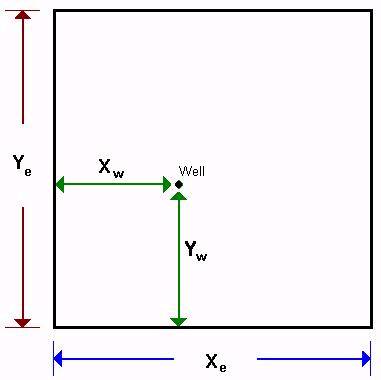
The Radial Model is actually a homogeneous rectangular reservoir model, with a vertical well located anywhere inside. The model is analytical and uses Green’s functions and method of images to calculate a fully integrated wellbore pressure history from early-time, through transition and into boundary dominated flow.

The model incorporates storage and skin effects. Rate dependent (turbulence) skin can also be accommodated (using a semi-analytical method) by entering a "D" turbulence factor.

The x and y dimensions of the reservoir can be set to any value above zero, and location of the well may be set to anywhere within the reservoir boundaries.

Pseudo-time is used for gas wells, to accommodate changing gas compressibility with reservoir pressure.

Parameters

Pi = initial pressure

k = permeability

h = net pay

s = skin (may be left blank)

D = turbulence factor (may be left blank)

C_D = storage coefficient (may be left blank)

x_e = reservoir length

y_e = reservoir width

x_w = x position of well within reservoir

y_w = y position of well within reservoir

O_IP = original gas/water/oil in place

Area = extent of reservoir

Models - Horizontal

Rectangular reservoir with a horizontal well located anywhere inside.

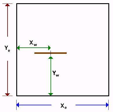
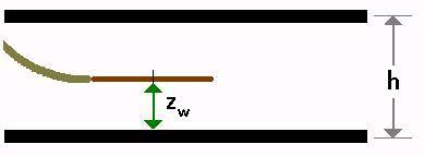
The Horizontal Well Model is a homogeneous rectangular reservoir model, with a horizontal well located anywhere inside. The model is analytical and uses Green’s functions and method of images to calculate a fully integrated wellbore pressure history from early-time, through transition and into boundary dominated flow.

The model incorporates storage and skin effects. Rate dependent (turbulence) skin can also be accommodated (using a semi-analytical method) by entering a "D" turbulence factor.

The model allows three dimensional anisotropy, providing inputs for permeability in the x, y and z directions. The effective wellbore length and stand-off height are also be included as model inputs.

The x and y dimensions of the reservoir can be set to any value above zero, and location of the well may be set to anywhere within the reservoir boundaries, provided the horizontal wellbore does not overlap any of the boundaries. Thus, it is possible to model the combined effects of horizontal wells and boundary flow in any number of different geometrical configurations.

Pseudo-time is used for gas wells, to accommodate changing gas compressibility with reservoir pressure.

Parameters

P_i = initial pressure

k_x, k_y, k_z = permeability in the x, y and z directions

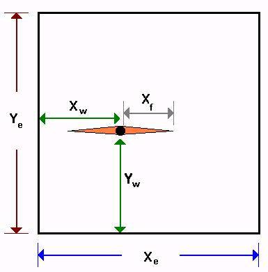
x_f = fracture half-length

L_e = effective wellbore length

z_w = z position of horizontal well within reservoir

s = skin

D = turbulence factor (also known as non-Darcy coefficient or turbulence skin effect)

C_D = wellbore storage coefficient

x_e = reservoir length

y_e = reservoir width

x_w = x position of well within reservoir

y_w = y position of well within reservoir

O_IP – original gas/water/oil in place

Area – extent of reservoir

Models - Fracture

Rectangular reservoir with a vertical infinite conductivity fracture located anywhere inside.

The Fracture Model is a homogeneous rectangular reservoir model, with a vertical hydraulic fracture (of infinite conductivity) located anywhere inside. The model is analytical and uses Green’s functions and method of images to calculate a fully integrated wellbore pressure history from early-time, through transition and into boundary dominated flow.

The model incorporates storage effects. Fracture half-length and fracture face skin may be specified by the user, also. Rate dependent (turbulence) skin can also be accommodated (using a semi-analytical method) by entering a "D" turbulence factor.

The x and y dimensions of the reservoir can be set to any value above zero, and location of the well may be set to anywhere within the reservoir boundaries, provided the fracture does not overlap any of the boundaries. Thus, it is possible to model the combined effects of fracture and boundary flow in any number of different geometrical configurations.

Pseudo-time is used for gas wells, to accommodate changing gas compressibility with reservoir pressure.

Parameters

P_i = initial pressure

k = permeability

x_f = fracture half-length

sc = choke skin (may be left blank)

D = turbulence factor (may be left blank)

C_D = storage coefficient (may be left blank)

x_e = reservoir length

y_e = reservoir width

x_w = x position of well within reservoir

y_w = y position of well within reservoir

O_IP = original gas/water/oil in place

Area = extent of reservoir

Models - Composite

A circular reservoir formed of concentric regions with a vertical well located at the center. The following schematic shows three regions, each with their own net pay value.

The composite model is composed of homogeneous concentric rings, with a vertical well located at the center. 

The model is analytical and calculates a continuous sandface pressure history from early-time, through transition and into boundary dominated flow. 

The model incorporates storage and skin effects. Rate dependent (turbulence) skin can also be accommodated (using a semi-analytical method) by entering a "D" turbulence factor.

The outer radius (r_o) for each ring can be set to any value that is greater than the r_o value for an inner ring. It is also possible to remove regions until all that remains is one region. Each region can have its own net pay (h).

Pseudo-time is used for gas wells, to accommodate changing gas compressibility with reservoir pressure.

Parameters

P_i = initial pressure

k = permeability

h = net pay

s = skin (may be left blank)

D = turbulence factor (may be left blank)

C_D = storage coefficient (may be left blank)

r_o = region outer radius

O_IP = original gas/water/oil in place

Area = extent of reservoir

Legacy Transient Reservoir

The Legacy Transient Reservoir models used in Piper are an approximation of the true analytical models.  In many cases the approximation, which does not incorporate superposition, has proved to be sufficient.  Note that the legacy transient well models will not match results from RTA for the same model type.

The Legacy Transient Reservoir model is defined by a number of parameters that determine the rate response of a reservoir to changes in pressure, such as permeability, porosity and skin (a full list is discussed below in the Required Input section). The Legacy transient well pool is a single well pool that behaves on the basis of tank type depletion.

A Transient Reservoir is illustrated pictorially below:

 

Piper allows for one of two boundary conditions to be associated with the reservoir; a radial finite boundary reservoir or infinite acting reservoir. The finite boundary reservoir option assumes a 'no-flow' boundary at the reservoirs extent whereas the infinite reservoir does not.

The reservoir may also be defined as either homogeneous through its extent, or as consisting of two regions, each with distinct properties of permeability and net pay. In Piper, a transient reservoir consisting of two regions is called a composite reservoir.

Required Input for a Transient Reservoir

The properties required to use the Transient Reservoir in Piper are as follows:

• Drainage Area
• Permeability
• Net Pay
• Distance to Boundary
• Total Porosity
• Skin Damage
• Wellbore Radius
• Water Saturation

Permeability

The permeability of a reservoir is a measure of the ability of a fluid to flow through rock as a function of pressure. Permeability is a property of the rock and is independent of the type of fluid. This means that the absolute permeability of a rock is the same whether the fluid traveling through it is oil, gas or water. In a petroleum reservoir, the rock is usually not fully saturated with a single phase fluid. Generally saturations in the reservoir rock will consist of different amounts of gas, oil and water. These saturations will change the effective permeability of the rock.

Piper requires the input of Permeability for transient wells.

Net Pay

This is the thickness of the formation that contributes to the flow of fluids. It is determined from logs or core, and can be different from the gross pay or the perforated interval. In the case of inclined wellbores in dipping formations, the net pay is measured perpendicular to the angle of dip.

Piper requires the input of Net Pay for transient wells.

Distance to Boundary

The distance to the boundary refers to the radial distance within the transient reservoir where reservoir properties (such as permeability, net pay, porosity and compressibility) and fluid parameters (such as viscosity) remain constant. Once the parameters appear to change, the limits of that zone have been reached.

In Piper the distance to boundary only needs to be defined for composite transient wells. For homogeneous finite transient wells, the distance to boundary is calculated directly from the area input. For infinite wells the distance to boundary is not required.

Total Porosity

The total porosity is the percentage occupied by the pore space, no matter what fluids are contained in the pore space. It is obtained from core or log analysis.

Most pressure transient analyses assume that the total porosity is filled with a single phase fluid, such that the total porosity equals the porosity to that specific fluid. In reality this is rarely the case, and the total porosity is usually filled with a mixture of oil, gas and water.

The total porosity has only a small effect during transient flow analysis but it has a significant effect during pseudo-steady state flow.

Piper requires the input of Total Porosity for transient wells.

Total Compressibility

In a reservoir, which consists of rock and pore space occupied by oil, water and/or gas, the total compressibility is the sum of several components. It takes into account the oil saturation, oil compressibility, water saturation, water compressibility, gas saturation, gas compressibility and the rock compressibility:

The compressibility of oil, water and the formation are of the same order of magnitude (10-6 1/psi) whereas the compressibility of gas is one or two order of magnitude larger. Therefore, if there is any gas present in the reservoir, the total compressibility is dominated by the gas compressibility component.

In transient flow analysis, the total compressibility has only a small effect. However, it has a significant effect during pseudo-steady state flow.

Piper requires the input of Total Compressibility for transient wells.

Skin Damage

The skin effect is a measure of the amount of damage or improvement to the formation in the vicinity of the wellbore.

Damage can be caused by drilling fluids, migration of fines, invasion, and results in a reduced permeability near the wellbore and a positive skin. The magnitude of the positive skin effect is generally 0 to 50 but can be as high as 200.

Improvement can be caused by acidizing or fracturing the formation and results in an increased effective permeability near the wellbore and a negative skin. The magnitude of the negative skin effect is generally 0 to -5.

The skin effect is a dimensionless quantity. It is defined as the difference between the "actual" and "ideal" dimensionless pressure drop in a reservoir.

An alternative concept to the skin effect is the "effective wellbore radius". This states that a well with a negative skin is equivalent to a well with a larger wellbore radius, while a well with a positive skin is equivalent to a well that has a smaller "effective wellbore radius".

Piper requires the input of Skin Damage for transient wells.

Wellbore Radius

In real life, the area of contact between the wellbore and the formation is rarely cylindrical. It depends on the perforations and is also affected by the type of perforating gun, casing, cement (see figure below).

 

Use of a Material Balance and Transient Wells

Transient wells are associated with both reservoir characteristics defined in the Transient Well editor, as well as characteristics defined the Pools editor.

Within the Pools editor, the Original Gas is Place of a Transient well is calculated from the Transient characteristics that are defined in the Transient Well editor. For a infinite pool transient well, this column will be left blank.

The cumulative production of a transient well can be defined in the pools menu. However, if a cumulative production is defined, it should be done so by defining a corresponding start date for the well in the Transient Well editor. A transient well that has associated with it a cumulative production but not a backdated start date, or conversely has a backdated start date but no cumulative production, will result in a mismatch between the material balance and the transient production. The results of this sort of mismatch are unrealistic and should be avoided.

Using Wellbores with Transient Wells

Piper now allows for wellbores to be associated with transient wells. The integration of a wellbore into a transient well will allow for the geometry of the wellbore to affect the well performance. Probably the most significant impact of this functionality is if the user elects to turn either the Turner or Coleman correlation on (found within the wellbore descriptions editor). With the selection of either the Turner or Coleman correlation, the ability of the well to lift liquids will be considered. In the event that the well cannot lift liquids, the well will load with liquids, following the loading procedure described in the wellbore tuning section of this Help.

Using Piper with Pressure Transient Analysis Software

Care must be taken when comparing results of Piper transient wells to the results of pressure transient analysis software. The results obtained by Piperare based on pressures obtained at the wellhead. Thus, they take into account the effect of pressure losses within the wellbore. This is in contrast to PTA software programs, which deal directly with pressure at the sandface.

Use of Pseudo pressure for Transient Wells

Piper the transient reservoir model has been modified to account for the effects of pseudo pressure. Previous versions of Piper used an approximation, the P-squared method, to estimate the change in pressure and compressibility with depth. The result of this change is that Piperwill model transient wells more accurately.

Because of the change introducing the use of pseudo pressure, transient wells defined in previous versions of Piper should be used in the version 5.800 release with caution. While for the general application of transient wells the change to using pseudo pressure should produce more accurate results, in cases where transient wells were being used to approximate a particular profile, the resultant profile in version 5.800 will have changed from what was calculated in previous versions.

Terminology

Cum Gas-to-Date

This is the cumulative production from the pool up to the forecast start date. When the Cum Gas to Date is subtracted from the Original Gas-In-Place, the remaining gas-in-place is obtained and current shut-in reservoir pressure can be obtained for use in the deliverability calculations.

Sandface C

The equation governing the Inflow Performance Relationship is known as the Rawlins-Schellardt back pressure equation. It is a relationship that can be applied to all gas wells and is independent of reservoir drive. It is generally derived from AOF or Inflow performance testing.

Where:

q = C x (PR2- Pf2)n
q – flow rate, MMscfd or m3
C – constant, MMscfd/(psi2)n or (m3/kPa2)n
n – turbulence of flow, dimensionless
PR – reservoir pressure, psia or kPaa
Pf – flowing pressure, psia or kPaa

There are no limits on the range of the allowed value of the constant "C" due to the complicated interaction between C, AOF, n and pressure. Be aware however, that systems can be sensitive to changes in "C" and that extreme values of "C" can result in extremely large deliverability potentials which can cause system instabilities.

Sandface n

The inverse slope on the back pressure plot, "1/n", describes the turbulence of the flow rate. An "n" value equal to 1 describes the laminar flow (no turbulence) and an "n" equal to 0.5 describes a fully turbulent flow. This value is dependent on the location of measurement. Values for "n" are valid only between 0.5 and 1.0

Input values less than 0.5 are automatically defaulted to 0.5 upon choosing OK to close the Well Deliverability Editor. Similarly, values greater than 1.0 are automatically defaulted to 1.0.

Initial Reservoir Pressure

The initial pressure measured at the mean Pool Depth. It is the starting point for the pool material balance calculation. This pressure, minus depletion caused by produced gas, equals the remaining reservoir pressure which is used in the deliverability calculations.

UNITS: psia (kPaA)

DEFAULT: 0

Original Gas-In-Place (OGIP)

This is the original volume of raw gas contained in the pool. When the Cumulative Gas-to-Date (raw) is subtracted from this number, the remaining gas-in-place is obtained. The Original-Gas-in-Place is obtained from volumetric (geological) calculations or pressure/production information.

Reservoir Depth

The depth from the wellhead to the pool datum. In gas reservoirs, because the reservoir hydrostatic pressure variation is negligible, the Pool Depth can be taken to be the average of the Mid-Point of Perfs of all the wells in that pool.

Note that Piper requires that e either the Pool Depth or the Mid-Point of Perfs must be entered. Also note that the Pool Depth and the Mid-Point of Perfs will default to one another if only one of the two values is entered.

Reservoir Remarks

This field allows for the entry of pool specific remarks. Remarks are shown on the gathering system map if selected for display.

UNITS: None

DEFAULT: None

Reservoir Temperature

The Reservoir Temperature is the average reservoir temperature. This value is not critical to the calculations. It affects the "Z-factor" calculations in the material balance equation. If wellbore calculations are being performed, then the Reservoir Temperature is used in calculating the temperature gradient in the wellbore.

Recovery Factor

The Recovery Factor specifies the percentage of recoverable reserves. The Recovery Factor should be used for a non-linear reservoir model such as the Connected Reservoir model or the Water Drive model. In these cases, the models may not properly account for late-time depletion effects. A Recovery Factor can be used to eliminate the possibility of over-predicting the late time gas production of such a reservoir.

Reservoir Pressure

This is the average pressure encountered in a reservoir. This is a function of the hydrocarbon fluid, water and rock properties in the reservoir. A higher reservoir pressure tends to increase the deliverability of a well.

Surface Loss

Surface loss in the case of the pool refers to the percentage of production is lost. This may be by venting, leaks, fuel gas or by a number of other means.

Gas Composition

The Gas Composition editor allows you to enter Gas Gravity, Acid Gases (CO2, H2S) and Inert Gases (N2) concentrations on a pool wide basis. If these items are omitted the program uses the Default Gas Properties.

However, if you select gas composition tracking (under Options main menu, Forecast sub menu), you can input a detailed pool composition.

Gas Gravity

Gas Gravity is the molar mass (molecular weight) of the natural gas divided by the molar mass of air (28.94). It ranges from 0.55 for dry sweet gas to approximately 1.5 for wet, sour gas. The Gas Gravity is readily obtained from any laboratory gas analysis.

In Piper, Gas Gravity affects three variables namely super-compressibility (Z-factor), gas viscosity, and gas density.

The effects on super-compressibility and viscosity are not very significant. However, the effect on density is significant in two ways. It affects the friction pressure drop to some extent, but it affects the hydrostatic pressure drop directly - i.e. doubling the Gas Gravity doubles the density and therefore doubles the hydrostatic pressure drop. Thus Gas Gravity affects calculations in vertical pipe segments far more than in horizontal segments. This becomes significant if wellbores are modeled under the Advanced option.

UNITS: None

DEFAULT: 0.65

Carbon Dioxide (CO2)

Concentration of Carbon Dioxide in the gas stream. It has an effect on the calculation of "Z-factor". In addition, it is a component to be included when estimating Surface Loss.

UNITS: Percent (%)

DEFAULT: 0

• Molecular weight: 44.01 kg/kmol
• Appearance: colorless gas
• Melting point: -56.6°C
• Boiling point: -78°C
• Gas Density: 1.977 kg/m3

Hydrogen Sulfide (H2S)

Concentration of Hydrogen Sulfide in the gas stream. It has an effect on the calculation of "Z-factor". In addition, it is a component to be included when estimating the Surface Loss.

UNITS: Percent (%)

DEFAULT: 0

• Molecular weight: 34.08 kg/kmol
• Appearance: colorless gas
• Melting point: -85.6°C
• Boiling point: -60.3°C
• Liquid Density: 993 kg/m3
• Gas Density: 1.496 kg/m3

Nitrogen (N2 )

Concentration of Nitrogen in the gas stream. It has an effect on the calculation of "Z-factor".

UNITS: Percent (%)

DEFAULT: 0s

• Molecular weight: 28.01 kg/kmol
• Appearance: colorless gas
• Melting point: -209.9°C
• Boiling point: -195.8 °C
• Gas Density: 1.250 kg/m3
• Liquid Density: 805 kg/m³

Methane (C1 )

Concentration of methane in the gas stream. This is considered to be the main produced hydrocarbon in most cases

UNITS: Percent (%)

DEFAULT: 100%

• Formula: CH4
• Molecular weight: 16.04 kg/kmol
• Appearance: gas
• Melting point: -182.5 °C
• Boiling point: -161.5 °C
• Gas Density: 0.717 kg/m3
• Liquid Density: 425 kg/m³

Ethane (C2)

Concentration of ethane in the gas stream. It has an effect on the calculation of specific gravity.

UNITS: Percent (%)

DEFAULT: 0

• Formula: C2H6
• Molecular weight: 30.07 kg/kmol
• Appearance: gas
• Melting point: -183.3 °C
• Boiling point: -88.7 °C
• Gas Density: 1.357 kg/m3
• Liquid Density: 548 kg/m

Propane (C3)

Concentration of propane in the gas stream. It has an effect on the calculation of specific gravity.

UNITS: Percent (%)

DEFAULT: 0

• Formula: C3H8
• Molecular weight: 44.11 kg/kmol
• Appearance: gas
• Melting point: -189.9°C
• Boiling point: -42.2°C
• Gas Density: 1.858 kg/m3

Butane (C4 or nC4)

Concentration of butane in the gas stream. It has an effect on the calculation of specific gravity.

UNITS: Percent (%)

DEFAULT: 0

• Formula: C4H10
• Molecular weight: 58.14 kg/kmol
• Appearance: gas
• Melting point: -138°C
• Boiling point: -0.6°C
• Gas Density: 2.499 kg/m3

Isobutane (iC4)

Concentration of isobutane in the gas stream. It has an effect on the calculation of specific gravity.

UNITS: Percent (%)

DEFAULT: 0

• Formula: C4H10
• Molecular weight: 58.14 kg/kmol
• Appearance: gas
• Boiling point: -10.2°C
• Gas Density: 2.467 kg/m3

Pentane (C5 or nC5)

Concentration of pentane in the gas stream. It has an effect on the calculation of specific gravity.

UNITS: Percent (%)

DEFAULT: 0

• Formula: C5H12
  Molecular weight: 72.17 kg/kmol
  Appearance: liquid
  Melting point: -130°C
  Boiling point: 36°C
  Liquid Density: 626 kg/m³

Isopentane (iC5)

Concentration of isopentane in the gas stream. It has an effect on the calculation of specific gravity.

UNITS: Percent (%)

DEFAULT: 0

• Formula: C5H12
• Molecular weight: 72.17 kg/kmol
• Appearance: gas

Hexane (C6)

Concentration of hexane in the gas stream. It has an effect on the calculation of specific gravity.

UNITS: Percent (%)

DEFAULT: 0

• Formula: C6H14
• Molecular weight: 86.178 kg/kmol
• Appearance: liquid
• Melting point: -95.4 °C
• Boiling point: 68.7 °C
• Gas Density: 659 kg/m³

Heptane (C7++ )

Concentration of hydrocarbons with a molar weight equal to or greater than heptane in the gas stream. It has an effect on the calculation of specific gravity.

UNITS: Percent (%)

DEFAULT: 0

• Formula: C7H16 (Heptane)
• Molecular weight: 100.23 kg/kmol
• Appearance: gas
• Melting point: -91°C
• Boiling point: 98°C
• Liquid Density: 684 kg/m³

Water (H2O )

Water is considered in several cases: static liquid columns, water influx into a reservoir, and liquid-gas ratios.

• Molecular weight: 18.02
• Appearance: colorless liquid
• Melting point: 0.0 °C
• Boiling point: 100.0 °C
• Gas Density: 0.600 kg/m3
• Liquid Density: 1000 kg/m³